|
|
|||||||||
|
||||||||||
|
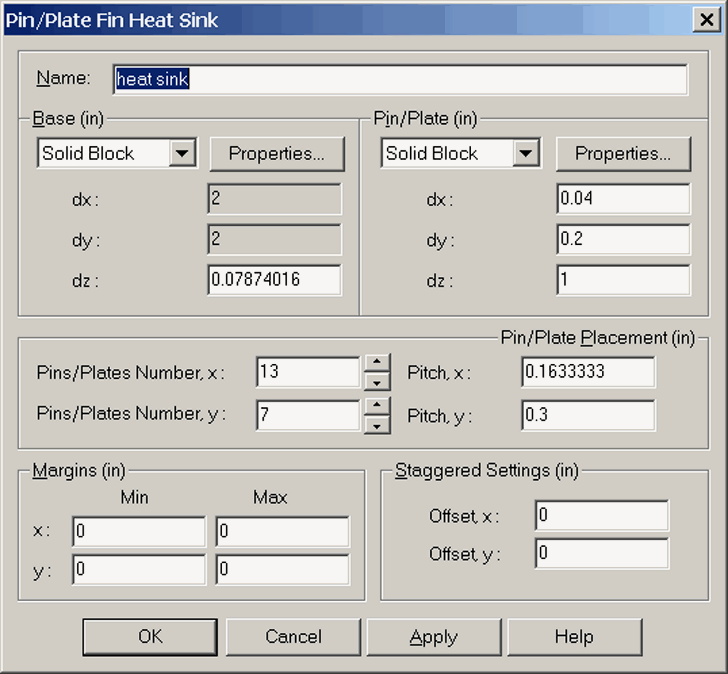
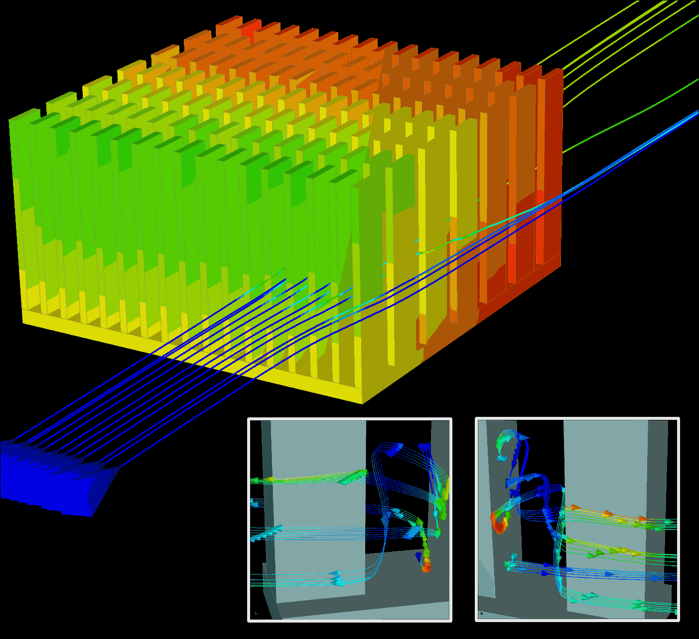
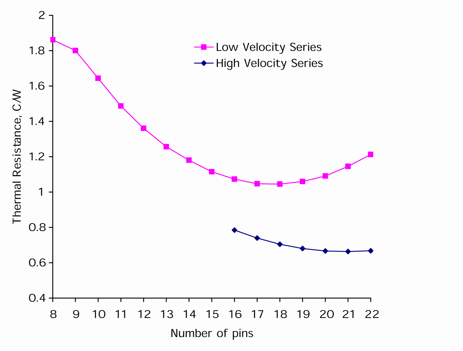
Engineers wrestling with thermal problems are familiar with constrained optimizations find a minimum size or weight, or both, for a device without reducing its performance, and usually without adding fans. From a mathematical standpoint, this involves finding the extreme value of a function under specified constraints. But standard optimization algorithms dont work well in thermal CFD cases. Heres why. Standard optimization procedures involve quantitatively defining what is to be optimized and forming a so-called objective function. It also involves specifying the variables that influence the objective function. In the following example, optimizing a pin-fin heat sink, these variables may include height, shape, spacing, and material of the pins and base. The objective function can be the thermal resistance of a sink, a mass-normalized heat transfer coefficient, or an array heat transfer coefficient. Depending on the number of variables, the objective function could be a line (one parameter), a surface (two parameters), or an n-dimensional hypersurface (n parameters). Finding the deepest valley, or minimum, on an n-dimensional hypersurface is not easy.  The input table for creating a parametric model of a heat sink. The specified parameters are saved with the sink. In order to change the design, modify parameters and click OK or Apply the heat sink will be automatically rebuilt. For thermal cases, solving a CFD problem determines a single point on a potentially vast surface. Hence, to describe a curve with ten points it takes 10 CFD solutions. For two parameters at 10 points each, it takes 100 CFD solutions. And with n parameters 10 points each, 10 n CFD solutions. Considering that CFD solutions for complex problems may take hours, its easy to see that automatic optimization of the sort used in other applications is not yet feasible. What is feasible, however, and done every day, is optimization using CFD solutions guided by engineering experience and intuition. Similar to automatic optimization, the manual method requires formulating an objective or goal and identifying parameters that affect the objective. The user then creates a limited number of cases to probe the parameter space and evaluate the sensitivity of the objective function to selected variables. This is similar to statistical optimization methods except that the user's intuition and experience, rather than random number generators, help select cases to search for an optimal point. The example here uses the tools in Coolit software to manually optimize a heat sink. Parametric tools help build the cases while batch tools assemble cases into a batch process for parallel or sequential solution. The program can also extract solution results pertinent to most commonly used objective functions. To build the heat sink in this example, users would click on a heat sink icon. A generic design pops onto the screen with a dialog box listing its parameters. Modifying them customizes the heat-sink model which can be rotated and zoomed even while the box is open. After specifying the base case, the rest of the batch is generated by varying parameters, such as the size, material, and spacing of fins, and size and material. For example, to assign several base widths, a user could type 2, 2.5, and 2.9 in. into that field. For this example, however, the material is aluminum 6061-T6, the base size is fixed at 2-in. X 2 in. X 0.0787 in., and pins are 1 in. X 0.4 in. X 0.02 in. There are seven pins to a row. A constant 10-W heat flux flows through the entire bottom surface. The variables will be the number of fins in the cross-flow direction at flow rates between 9.2 and 18.4 cfm. Heat-sink performance depends on, of course, its characteristics, and the environment. But unless one deals with a fully shrouded sink, the flow through it is determined by the interplay between the flow resistance of the entire system and the heat sink. If possible, initial cases should attempt to bracket the extreme values of the objective function to guide further studies and produce the least number of follow up cases. Initial studies usually run with more cases, so it is preferable to select a subset of cases, which will run faster, thereby reducing the number of more complicated cases to run later. Applying this strategy to the example calls for first analyzing cases with lower velocities. After finding an initial optimal fin spacing, we would use the information to shorten studies of higher velocities, which normally require more time to compute.  Flow around a heat sink used in this study. The heat sink and streamlines are painted in temperature. The insets show flow pattern between two pins. The pins in the insets are painted in solid color and streamlines are painted in temperature. Its easy to build the base case because all the components are available in the thermal software. Additional details are added by selecting from menus or filling in tables. The finite volume grid and solver parameters are usually set automatically. So after specifying geometry and materials, simply press the Go button to solve the problem. To ensure result consistency, some programs let users specify a minimum number of grid cells that define a pin as well as passages between them. Solver variables affect only the convergence rate, or how fast one gets to a solution, but not its accuracy. This example uses default settings for both the grid and the solver. Running ten cases makes it important to have a solver that reliably converges without user intervention. Too much intervention makes optimization studies near impossible. For instance, older programs might require stopping and restarting the solver after adjusting convergence controls, or turning solved equations on and off. The study starts by running the base case with 10 pins and an inlet flow of 9.2 cfm to get an idea of the needed time to solve the problem and to make sure there are no mistakes in the set up. If the case works well, clone it with different numbers of pins and set up a batch process to run them together. The initial case contained about 87,000 grid cells and it took 173 iterations to run in under 25 min. on a Pentium III 800 MHz PC. After checking case results, we set up 12 more cases to consider 11 to 22 pins. This can run overnight.  Results for the first twelve runs in Coolit from Daat Research Corp., show that heat dissipation maximized at 18 pins for the 9.2 CFM flow rate. The experiment for 18.4 CFM flow, was started with a 19 pin heat sink and its optimum is reached for a heat sink with 21 pins. The plot shows extra points for each study to better illustrate the trends. The first 12 runs show results which include the heat resistance based on the temperature rise in the sink's base as a function of the number of pins in cross flow. It is a smooth curve with the minimum at 18 pins. From hydrodynamic considerations, it is clear that higher inlet velocities will put the optimum point higher, i.e. it will require more pins. Therefore, to save time, we can start high-velocity experiments at 19 pins. Also, we will use only one more velocity the maximum rate specified, or 18.4 cfm, on the assumption that once we have the optimal configuration for bounding values, the optimum for other velocities should fall in between. Despite being plausible, the assumption of monotone behavior (although valid in this case) is not always correct and generally has to be tested. Recognizing that we are not far from the optimal point, we run only five experiments starting from the 19 pin-fin heat sink. The optimum point in the second batch is at 21 pins. All cases in the later study started with lower-velocity solutions for corresponding heat sinks, which helped reduce the solution time. The heat sink with 19 pins is selected as optimal using results from the two computer series, and assuming that inflow velocities within the specified range are equally likely. To summarize: Build a representative case and run it to verify the set up, grid, and modeling assumptions. The main criteria for selecting the first variable is the potential to use the information from the first study to minimize the number of cases for other parameters and also the relative simplicity of cases to minimize solution time for the first series, which is often the longest. With satisfactory results, serialize the case and prepare a batch process. In multiparameter studies, select a single parameter to start. Analyze results from the first series to guide the direction of the follow-up search.
|
||||||||||
|
||||||||||