Turbulence is associated with the presence of both spatial and temporal random fluctuation in the flow
field. It develops gradually from laminar flows that display regular variations in both space and
time, through a sequence of instabilities, which develop as the Reynolds number (Re), which measures
the ratio of the inertia to viscous forces of flow, is increased. Turbulent fluctuations significantly
increase the intensity of the momentum and heat transport. Typical values in electronics are between
10 to 100 times the rate of the corresponding molecular transport rates. Increasing the rate of heat
transfer is normally a positive development for electronics cooling, while increasing the momentum
transport is not, as it results in higher wall shear stress and hence higher pumping requirements.
Under these conditions neglecting turbulence is not an option.
By now it has been definitively established that the Navier-Stokes equations solved by CFD
programs, do describe turbulence. That is in theory, you don't need any additional equations to model
turbulent flows. In practice, the turbulence is associated with very small-scale fluid motions
(eddies). Thus the ratio of the smallest length scale to the size of domain in turbulent flow is
proportional to Re-3/4. That is, even for very slow turbulent flows with the Reynolds
number of a few thousands, grids on the order of 1,0003 are required. Such direct
simulations, therefore, are of purely academic interest.
The only practical way to compute turbulent flows that exists today is to use turbulence models.
Most popular models use the eddy viscosity concept proposed by Boussinesq. This concept is based on
the analogy between molecular transport of momentum and heat and their turbulent transport by the
eddies. Using this approach one solves the ensemble-averaged Navier-Stokes equations and a model that
computes the eddy transport. Unlike the molecular viscosity and thermal conductivity, which are
strictly material properties of fluid, the eddy properties depend on the nature of the flow and vary
significantly over the solution domain.
As of now, there is no single turbulence model that works equally well across all flow types and
geometries. However, there are models that work better than others for specific flow conditions.
Coolit provides a choice of 4 turbulence models, which have been shown to work well in low Reynolds
number, buoyant flows encountered in electronics cooling applications. A comparison of several popular
models used by commercial codes and a Coolit model is presented in the paper on this web site.
When the flow is mixed, i.e. laminar, transitional, and turbulent regions coexist within the
solution domain, the decision whether to use a turbulence model is not obvious. It will depend on
location of important components. If all critical components are in turbulent region, for example,
next to the fan, the decision to use a turbulent model is clear. However, when they are in both
regions, the Coolit's eddy viscosity model without wall functions should be used. This model has been
shown to predict mixed flows with good accuracy.
In many problems the temperature field in components is steady (i.e. time-independent), while flow
in at least some areas of the modeled domain is time-dependent. For example, in many natural
convection problems, the rising plume often becomes unstable (time-dependent) or in forced convection
problems time-dependent vortex shedding occurs behind blunt objects. In such cases no steady state
solution exists and hence there is no convergence. Unless your interest is in obtaining accurate
resolution of time behavior of the unstable portion of the flow, solving such problems as
time-dependent is not a good idea. Normally the temperature inside components is steady and if your
objective is to find that temperature you have two options.
Solve the problem as laminar until solution residuals come to a stably oscillating pattern. You can
define the solution at that stage as "converged". Although the flow pattern in the oscillating portion
of flow is apparently periodically changing, the temperature in components does not. The second option
is to use the eddy viscosity turbulence model without wall functions to dampen the time-dependent
oscillations and force a steady state solution.
We know "critical" Reynolds numbers for several simple
geometries: flat plate, circular pipe, etc. Critical Reynolds number is
usually defined as the value above which perturbations present in the flow do
not decay. A more practical definition says that the flow with Re <
Recr is always laminar independently of the magnitude of
perturbations. Clearly, exceeding the critical Reynolds number does not imply
a turbulent flow. Thus, for example, the Recr for flows in
circular pipes is around 2,300. However, there were experiments that observed
turbulence in circular tubes starting at Re=50,000!
Another problem is that it is not clear how to define
Reynolds numbers in a complex geometry. In classical geometries, such as
pipes and flat plates, the definition of Re is straightforward; there is
usually only one velocity scale and one or two length scales to work with. In
a real-life geometry there could be tens or hundreds of such scales and the
quantity of the corresponding Reynolds numbers can grow proportionally
large.
On the positive side, note, that in most electronics
application flows maximum Reynolds numbers are on the order of 10,000. This
indicates that they are mostly laminar with possibly some patches of
turbulent and transitional flow.
We can suggest several practical guidelines to help determine the flow regime.
Flow is always turbulent near the fan. On the suction side, though, the turbulence zone can be
small.
Flows between closely spaced components and surfaces (such as PWBs) are almost always
laminar.
Expanding flow streams become turbulent at relatively low Reynolds numbers, while converging
streams require much higher Re to become turbulent.
If in doubt, or you know that the flow is mixed, use the Coolit's eddy viscosity model without wall functions. It has a good track record in correctly predicting such flows under a variety of flow conditions.
Coolit provides 4 different turbulence models: algebraic, differential, eddy viscosity with and
without wall functions. The models using wall functions are most appropriate for fully developed
turbulent flows. The do include a mechanism for switching to laminar flow where little turbulence is
detected. However, this mechanism is not very reliable. For better accuracy in mixed flows, the
turbulence model without wall functions should be used.
Since the simpler models, such as the algebraic model, are much faster to compute, for important
analyses, compare its prediction with the more accurate eddy viscosity models. If the predicted
parameters in important areas are within acceptable limits, you can safely use the faster model. In
terms of accuracy, the eddy viscosity models are the most accurate, followed by the differential, and
then algebraic models.
As a general statement it is correct to say, that RANS (Reynolds-averaged Navier-Stokes) equations
used by all commercial CFD codes, cannot predict transition/relaminarization under general
circumstances. The only methods that can currently do that for are direct Navier-Stokes simulations
(DNS) and large eddy simulation (LES) techniques. Delving into DNS/LES is beyond the scope of this
note, but it is safe to say that, for the next two decades at least, due to enormous computational
requirements, these methods will be limited to academic environment for relatively simple problems.
In the early nineties, three turbulence models for RANS had appeared (Spalart-Allmaras, 1992,
Secundov, 1992, and Menter, 1993) that to some extent had the ability to predict both the transition
and relaminarization. The models could not consistently predict the exact location of relaminarization
in general problems, but some of them could be tuned to work well in specific classes of problems.
Moreover, even in circumstances where the exact location of relaminarization is missed, the models
would predict very low eddy viscosity values, consistent with laminar flow and hence sufficient for
engineering purposes.
In low Reynolds number flows, such as the ones in electronics cooling applications, the Coolit
model predicts very well both high and low turbulence areas through a careful balance of
dissipation/generation terms in the model equations. The Coolit model is also capable of predicting
the so called bypass transition to turbulence, that is, transition caused by contamination of laminar
boundary layers by external turbulence from, for example, fans; a scenario typical for a wide range of
electronic equipment.
Solve a problem on a given grid and obtain a solution at important locations. Refine the grid and solve the problem again. If the solution has not significantly changed the first grid was sufficient. Otherwise continue the grid refinement until the satisfactory grid independence is obtained.
Often it is important to resize enclosure from a specific side only. For example, you set up a case with a custom grid, solved it, and now you wish to reduce the spacing between the Xmin wall and interior components. If you use the Control Bar Size edit windows to modify the size or drag the enclosure side with the mouse, the enclosure will be resized from the Xmax side. Moving components towards the left (Xmin) wall will destroy your grid.
Coolit provides two solutions to resize enclosure from Xmin side. If you want to use the mouse to resize enclosure, hold the Shift key while dragging the side. The enclosure will move Xmin towards your interior components. The second option is to use the Enclosure Properties dialog. Enter the new X-size and check the box next to it. When you click OK the enclosure will be resized from Xmin side.
As the problem is being solved, Coolit shows the Convergence Monitor - a 2D plot of
solution residuals vs. iteration number. In Coolit, the solution residual defines how far
the computed solution for a given variable (velocity components, pressure, and temperature)
deviates from steady state. Normally the solution is called "converged" when the residuals
for all the variables are less than 10-3.
In addition to residuals, Convergence Monitor displays plots of the temperature,
pressure, and velocity magnitude at Monitor Probe locations. Even if you have not created
Monitor Probes, it will display maximum and minimum values.
In most problems, which have a steady state solution, the convergence history consists of
relatively smooth curves going down until they drop below the specified convergence precision line. In
some problems, it never happens; in such cases we say that the problem does not converge. Two most
often encountered reasons for non-convergence are too closely spaced grids and problems which have no
steady state solution.
The convergence is affected by the closely spaced grids because computers use finite
precision for arithmetic and if the grid spacing is near the limit of computer precision,
severe convergence problems will occur. The important notion here is not the absolute
distance between grids, but rather the normalized distance, |xi-xi+1|
/ xi+1, where xi and xi+1 are coordinates of neighboring
grid lines. Coolit provides an automatic check for grid lines closer than 0.001, i.e.
|xi-xi+1| / xi+1 < 0.001, and reports them in the Listing
of Closely Spaced Components dialog, which can be view by clicking the Model Check button.
If grid lines closer than the specified limit are found Coolit will issue a warning.
If a case for which Coolit issued a warning does not converge, you should eliminate the
reported problems. This can be done either manually by moving and resizing components, so
that they line up or by specifying the Anchor Grid Tolerance in the Grid Settings|Parameters
dialog. The Tolerance should be greater than the largest of the offending distances listed
by Model Check. This can also be done automatically in the Model Check dialog by pressing
the Fix button.
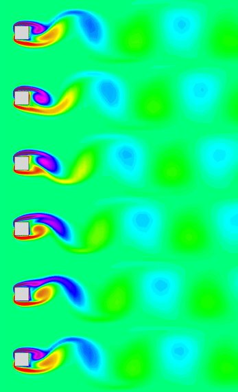
Another often encountered reason for non-convergence is when a flow develops
time-dependent flow patterns due to the instability. A common example of this phenomenon is
an oscillating wake behind an object as shown in the picture below. Such a periodic vortex
shedding produces a corresponding oscillations in the residuals, that measure the departure
of solution from steady state. You won't be able to find a steady state solution to this
laminar flow problem, because it does not exist.
Users have several options after recognizing that the wake's oscillations have little
effect on the temperature of the cylinder: accept the solution with oscillating residuals as
"converged"; use a turbulence model without wall functions to dampen the oscillations and
obtain a steady state solution, or solve the problem as time-dependent, obtain results over
a period, and average them. All three approaches are legitimate and produce similar results.
But unless you are writing a scientific paper, the third approach is not practical because
it takes a lot longer than the other methods. You can also sometimes reduce the magnitude of
the oscillating residuals by unchecking the Local Time Stepping option in the Solver
Settings|Expert Parameters dialog and reducing the Courant number.
Normally, you take the difference between the predicted value and the measured value and divide it
by the measured value. Here is an example: Ambient = 40C, predicted junction temperature for a chip
= 120C, measured = 110C. Error = (110-120)/110 = 9% However, if you use the Kelvin scale to report
temperature, you get: Ambient = 313K, predicted junction = 393K, measured = 383K Error =
(383-393)/383 = 3%. Obviously, the same data shouldn't give different errors.
To determine the error between Coolit predicted temperatures and measured values, you
need to look at the temperature rise above ambient:
in degrees Celsius:
Error = [(110-40)-(120-40)]/(110-40) = [70-80]/70 = 14%
or in degrees Kelvin:
Error = [(383-313)-(393-313)]/(383-313) = [70-80]/70 = 14%
The same rule applies when comparing computed predictions to each other (for instance, when
investigating the sensitivity of the computed temperature rise to the grid density).
In this case, the reference temperature rise is not a measured value. So you should use the average
temperature rise for all of the solutions to normalize the data. For example, two Coolit simulations
give a component temperature of 101C and 98C respectively. The ambient is 20C. The sensitivity is:
The standard non-dimensionalization does not work well with temperatures, because the Celsius and
Fahrenheit scales have "offsets" built into them that make zero Celsius or zero Fahrenheit not equal
to absolute (Kelvin) zero. When you take differences, as in equation, you subtract out the offset,
but it remains in the denominator and thus changes the result depending on which temperature scale
you use. The Kelvin scale does not have an offset (0 K = absolute zero) and therefore does not have
this problem.
Even in cases where the temperature is measured in Kelvin, using the standard
non-dimensionalization is usually inappropriate. Typically it is used only when the value of the
variable relative to zero is important. For example, if you are using Coolit to predict the pressure drop, dP,
across a heat sink at a fixed flow rate. In this case, dP across your heat sink is measured relative
to zero dP, so equation the standard non-dimensionalization is used to calculate the error.
In electronics cooling applications there is normally an ambient temperature,
Tambient, which dictates the lowest possible temperature for the problem. In such cases, that
ambient temperature is the reference and any errors in Coolit predictions for temperatures should be
calculated relative to Tambient:
The attached document provides empirical formulas
and detailed guidelines for specifying resistance parameters in Coolit Planar
Porous Resistance components.
The pressure losses in plate fin heat sink type of geometry are caused primarily by the shear
stress along the plate fins. Secondary contributions are the form drag created by the blunt ends of
the fins and the flow contraction and expansion into and out of the heat sink.
Before you grid the problem, you must select a flow model. There are three possibilities:
Case 1: The flow is laminar both inside and outside the heat sink. In this case, use the
Laminar model.
Case 2: The flow is laminar or transitional inside the heat sink and transitional or turbulent
outside. In this case, use the turbulent Eddy Viscosity w/o Wall Functions model.
Case 3: It is computationally prohibitive to resolve the velocity gradients in high Reynolds
number flows. In these cases, a wall functions model can provide good accuracy with a coarse
grid. In order for wall functions models to be accurate, y+ in the channels should be 30 or
greater. Create 2 cells in each channel, run your model, and view the y+ values in CoolPlot to
check for this condition.
For guidelines on determining whether the flow is laminar, transitional, or turbulent, see How to determine if flow is turbulent? When computing the Reynolds number
for flow in the duct before and after the heat sink use the hydraulic diameter of the duct as the
length scale.
Once you have selected your flow model, grid the problem manually according to the guidelines below
for each direction.
Perpendicular to the Fin Surfaces
Case 1: Use the Multiple Lines grid editing tools with an expansion factor of 1.2 or less to
grid the channels between the fins. Begin with a grid that has at least 1 grid cell in the
boundary layer computed from Hbl = 10*w/sqrt(Re10w). Here w is the distance
between fins, Re10w = Uave*10*w/n, Uave is the average
velocity in the channel, and n is the kinematic viscosity of air at the temperature and pressure
in your problem. Refine the grid at least twice and monitor the pressure drop solution for
change.
Case 2: For mixed flows that contain laminar, transitional, and turbulent flow regions, the
Eddy Viscosity w/o Wall Functions model can provide the best accuracy. As in the laminar case
above, the grid must be fine enough to resolve the gradients near the walls in the channels. The
non-dimensional parameter, y+, reported by CoolPlot provides a tool for evaluating the fineness of
the grid near the wall. Typically, y+ < 2 on channel walls should compute the pressure drop to
within 10%. Compute a solution with the default grid. View the results in CoolPlot and select the
y+ option in the Surfaces pull-down menu. View the surface of the interior plate fins to evaluate
the y+ value over the bulk of the fin surface (it may be useful to hide some fins and adjust the
range of the Color Palette). Use the Multiple Lines grid editing tools with an expansion factor
of 1.2 or less to refine the grid in the channels until the y+ value drops below 2 while
monitoring the pressure drop solution for change.
Case 3: It is computationally prohibitive to resolve the velocity gradients in high Reynolds
number flows. In these cases, a wall functions model can provide good accuracy with a coarse
grid. In order for wall functions models to be accurate, y+ in the channels should be 30 or
greater. Create 2 cells in each channel, run your model, and view the y+ values in CoolPlot to
check for this condition.
In the Flow Direction
For All Cases: In order to resolve the form drag and the developing boundary layer in the channel, you need to
have several cells stacked up near the entrances and exits of the channels. Use the Multiple Lines grid editing
tools with an expansion factor of 1.2 to create a grid with at least three cells in the first channel width before
and after the entrance to the channels and after the exit of the channels. As always, refine the grid at least
twice and monitor the pressure solution for change.
In the Fin Height Direction
For All Cases: Grid density in this direction does not have much effect on the solution inside the
channels.
The grid requirements for computing accurate temperature solutions are significantly lower
than that for the pressure despite the fact that the boundary layer thickness of velocity and
temperature are very close. Fortunately, resolving the temperature boundary layer is not necessary
in order to predict accurate temperature in both the solid and the air. Here's why:
a. Lets assume that a solid object generates Q Watts of power. A good CFD program should
conserve momentum, mass, and energy EXACTLY. Such a program would then compute that the entire Q
is dissipated in the air, independent of the grid used. This is an integral property, i.e. the
property which is obtained by integrating around the solid's surface of differential heat fluxes
for each surface grid cell. And even though the individual fluxes may not be very accurate (that
would require resolving the boundary layer) their integral would exactly match Q.
b. We have established that in a well-written CFD program, the total generated power is
dissipated in the air independently of the grid or ambient conditions. However, the temperature of
our solid object depends not only on Q but also on the temperature of the air around it.
Specifically, in a CFD model, it depends on the temperature of the air in the first cell outside
the solid. In most cases, the default grid is sufficiently fine to compute the bulk airflow
velocity and temperature around a solid body.
This is in contrast to the situation for pressure drop where you need to have an accurate
prediction of the derivative, or rate of change, of the velocity. This requires a much finer grid.
For example, in a short channel with a Reynolds number of 1600 (based on channel width), 8 cells
were required in the channel to get within 10% error for the pressure drop; only 3 were required
to get within 10% error for the average temperature of the walls.
c. Finally, in (b) we assumed that the bulk airflow around the solid body is computed
correctly. However, when you have a fan curve, the flow rate depends on the pressure drop. In some
cases, such as ducted heat sinks, predicting the pressure drop requires resolving velocity
boundary layers. However, in most cases, the pressure drop through a system is determined by form
drag over a number of solid bodies. In these cases, a coarse grid is all that is required to
resolve this form drag and correctly predict pressure drop and thus flow rate.
In all cases, you should refine the grid at least twice and compare the results. If the
solution is still changing significantly, continue to refine the grid.
We have done extensive benchmarking of Coolit and it can compute pressure drop in channels
with contractions and expansions to within a few percent. Empirical formulas, such as from
Idelchik's handbook, predict expansion/contraction losses to within an order of magnitude only.
Consider the classic experiment by Jovic, S. and Driver, D.M., NASA Technical Memorandum
108807, 1994, where they measured the pressure drop in an expansion. For a channel with a 5-fold
expansion and Re=5,000 the experiment predicted the pressure loss coefficient of 0.21. Using
Idelchik's formulas you get 0.028 - 7.5 times less than experiment.
For contraction case, we used the data by Moss, W. D. and Baker, S., Aeronautical Quartery,
August 1980, pp. 151-172. For a channel with a 10-fold constriction and Re=47,740 the experiment
predicted the pressure loss of 0.3; Idelchik - 0.0902.
When using Coolit to compute benchmark quality results, you should refine the grid at least
twice and compare the results. If the solution is still changing significantly, continue to refine
the grid.